Paired integration and query-to-reference mapping

In this tutorial, we demonstrate how to use Multigrate’s integration module for paired integration, i.e. reference building, and mapping on the query onto the built reference. We will use NeurIPS 2021 CITE-seq dataset [LBC+21].

import sys

# if branch is stable, will install via pypi, else will install from source
branch = "latest"
IN_COLAB = "google.colab" in sys.modules

if IN_COLAB and branch == "stable":
    !pip install multigrate[tutorials]
elif IN_COLAB and branch != "stable":
    !pip install muon
    !pip install --quiet --upgrade jsonschema
    !pip install git+https://github.com/theislab/multigrate

import anndata as ad
import multigrate as mtg
import muon
import scanpy as sc
import scvi
import warnings

warnings.filterwarnings("ignore")

scvi.settings.seed = 0
print("Last run with scvi-tools version:", scvi.__version__)

Last run with scvi-tools version: 1.4.0.post1

Data loading

The data contains 90,261 bone marrow mononuclear cells. This CITE-seq (i.e. paired gene expression and surface protein adundance) dataset was generated at 4 different sites introducing some batch effect. After the quality control performed by the authors, the data contains measurements from 13,953 genes and 134 proteins.

data_path = "GSE194122_openproblems_neurips2021_cite_BMMC_processed.h5ad"

try:
    adata = sc.read_h5ad(data_path)
except OSError:
    !wget 'ftp://ftp.ncbi.nlm.nih.gov/geo/series/GSE194nnn/GSE194122/suppl/GSE194122_openproblems_neurips2021_cite_BMMC_processed.h5ad.gz'
    !gzip -d GSE194122_openproblems_neurips2021_cite_BMMC_processed.h5ad.gz
    adata = sc.read_h5ad(data_path)

adata

AnnData object with n_obs × n_vars = 90261 × 14087
    obs: 'GEX_n_genes_by_counts', 'GEX_pct_counts_mt', 'GEX_size_factors', 'GEX_phase', 'ADT_n_antibodies_by_counts', 'ADT_total_counts', 'ADT_iso_count', 'cell_type', 'batch', 'ADT_pseudotime_order', 'GEX_pseudotime_order', 'Samplename', 'Site', 'DonorNumber', 'Modality', 'VendorLot', 'DonorID', 'DonorAge', 'DonorBMI', 'DonorBloodType', 'DonorRace', 'Ethnicity', 'DonorGender', 'QCMeds', 'DonorSmoker', 'is_train'
    var: 'feature_types', 'gene_id'
    uns: 'dataset_id', 'genome', 'organism'
    obsm: 'ADT_X_pca', 'ADT_X_umap', 'ADT_isotype_controls', 'GEX_X_pca', 'GEX_X_umap'
    layers: 'counts'

Data preparation

We subsample the data to speed up the training.

sc.pp.subsample(adata, n_obs=20000)
adata

AnnData object with n_obs × n_vars = 20000 × 14087
    obs: 'GEX_n_genes_by_counts', 'GEX_pct_counts_mt', 'GEX_size_factors', 'GEX_phase', 'ADT_n_antibodies_by_counts', 'ADT_total_counts', 'ADT_iso_count', 'cell_type', 'batch', 'ADT_pseudotime_order', 'GEX_pseudotime_order', 'Samplename', 'Site', 'DonorNumber', 'Modality', 'VendorLot', 'DonorID', 'DonorAge', 'DonorBMI', 'DonorBloodType', 'DonorRace', 'Ethnicity', 'DonorGender', 'QCMeds', 'DonorSmoker', 'is_train'
    var: 'feature_types', 'gene_id'
    uns: 'dataset_id', 'genome', 'organism'
    obsm: 'ADT_X_pca', 'ADT_X_umap', 'ADT_isotype_controls', 'GEX_X_pca', 'GEX_X_umap'
    layers: 'counts'

We split the data into the gene counts and protein counts.

rna = adata[:, adata.var["feature_types"] == "GEX"].copy()
rna

AnnData object with n_obs × n_vars = 20000 × 13953
    obs: 'GEX_n_genes_by_counts', 'GEX_pct_counts_mt', 'GEX_size_factors', 'GEX_phase', 'ADT_n_antibodies_by_counts', 'ADT_total_counts', 'ADT_iso_count', 'cell_type', 'batch', 'ADT_pseudotime_order', 'GEX_pseudotime_order', 'Samplename', 'Site', 'DonorNumber', 'Modality', 'VendorLot', 'DonorID', 'DonorAge', 'DonorBMI', 'DonorBloodType', 'DonorRace', 'Ethnicity', 'DonorGender', 'QCMeds', 'DonorSmoker', 'is_train'
    var: 'feature_types', 'gene_id'
    uns: 'dataset_id', 'genome', 'organism'
    obsm: 'ADT_X_pca', 'ADT_X_umap', 'ADT_isotype_controls', 'GEX_X_pca', 'GEX_X_umap'
    layers: 'counts'

adt = adata[:, adata.var["feature_types"] == "ADT"].copy()
adt

AnnData object with n_obs × n_vars = 20000 × 134
    obs: 'GEX_n_genes_by_counts', 'GEX_pct_counts_mt', 'GEX_size_factors', 'GEX_phase', 'ADT_n_antibodies_by_counts', 'ADT_total_counts', 'ADT_iso_count', 'cell_type', 'batch', 'ADT_pseudotime_order', 'GEX_pseudotime_order', 'Samplename', 'Site', 'DonorNumber', 'Modality', 'VendorLot', 'DonorID', 'DonorAge', 'DonorBMI', 'DonorBloodType', 'DonorRace', 'Ethnicity', 'DonorGender', 'QCMeds', 'DonorSmoker', 'is_train'
    var: 'feature_types', 'gene_id'
    uns: 'dataset_id', 'genome', 'organism'
    obsm: 'ADT_X_pca', 'ADT_X_umap', 'ADT_isotype_controls', 'GEX_X_pca', 'GEX_X_umap'
    layers: 'counts'

# to free memory
del adata

RNA preprocessing

Next, we log-normalize the raw counts and subset the RNA data to 2,000 highly variable genes.

rna.X = rna.layers["counts"].copy()

sc.pp.normalize_total(rna, target_sum=1e4)
sc.pp.log1p(rna)

n_top_genes = 2000
batch_key = "Site"

sc.pp.highly_variable_genes(rna, n_top_genes=n_top_genes, batch_key=batch_key, subset=True)
rna

AnnData object with n_obs × n_vars = 20000 × 2000
    obs: 'GEX_n_genes_by_counts', 'GEX_pct_counts_mt', 'GEX_size_factors', 'GEX_phase', 'ADT_n_antibodies_by_counts', 'ADT_total_counts', 'ADT_iso_count', 'cell_type', 'batch', 'ADT_pseudotime_order', 'GEX_pseudotime_order', 'Samplename', 'Site', 'DonorNumber', 'Modality', 'VendorLot', 'DonorID', 'DonorAge', 'DonorBMI', 'DonorBloodType', 'DonorRace', 'Ethnicity', 'DonorGender', 'QCMeds', 'DonorSmoker', 'is_train'
    var: 'feature_types', 'gene_id', 'highly_variable', 'means', 'dispersions', 'dispersions_norm', 'highly_variable_nbatches', 'highly_variable_intersection'
    uns: 'dataset_id', 'genome', 'organism', 'log1p', 'hvg'
    obsm: 'ADT_X_pca', 'ADT_X_umap', 'ADT_isotype_controls', 'GEX_X_pca', 'GEX_X_umap'
    layers: 'counts'

ADT preprocessing

We will use centered log-ratio (CLR) normalization for the ADT modality.

adt.X = adt.layers["counts"].copy()

muon.prot.pp.clr(adt)
adt.layers["clr"] = adt.X.copy()

Data setup

Next, we create one AnnData object from the RNA and ADT objects and specify which layers to use during training.

adata = mtg.data.organize_multimodal_anndatas(
    adatas=[[rna], [adt]],  # a list of anndata objects per modality, RNA-seq always goes first
    layers=[["counts"], ["clr"]],  # if need to use data from .layers, if None use .X
)
adata

AnnData object with n_obs × n_vars = 20000 × 2134
    obs: 'GEX_n_genes_by_counts', 'GEX_pct_counts_mt', 'GEX_size_factors', 'GEX_phase', 'ADT_n_antibodies_by_counts', 'ADT_total_counts', 'ADT_iso_count', 'cell_type', 'batch', 'ADT_pseudotime_order', 'GEX_pseudotime_order', 'Samplename', 'Site', 'DonorNumber', 'Modality', 'VendorLot', 'DonorID', 'DonorAge', 'DonorBMI', 'DonorBloodType', 'DonorRace', 'Ethnicity', 'DonorGender', 'QCMeds', 'DonorSmoker', 'is_train', 'group'
    var: 'modality'
    uns: 'modality_lengths'
    layers: 'counts'

The data comes from 4 different sites, so we select one of the sites as the query.

query = adata[adata.obs[batch_key] == "site1"].copy()
adata = adata[adata.obs[batch_key] != "site1"].copy()
(adata, query)

(AnnData object with n_obs × n_vars = 16433 × 2134
     obs: 'GEX_n_genes_by_counts', 'GEX_pct_counts_mt', 'GEX_size_factors', 'GEX_phase', 'ADT_n_antibodies_by_counts', 'ADT_total_counts', 'ADT_iso_count', 'cell_type', 'batch', 'ADT_pseudotime_order', 'GEX_pseudotime_order', 'Samplename', 'Site', 'DonorNumber', 'Modality', 'VendorLot', 'DonorID', 'DonorAge', 'DonorBMI', 'DonorBloodType', 'DonorRace', 'Ethnicity', 'DonorGender', 'QCMeds', 'DonorSmoker', 'is_train', 'group'
     var: 'modality'
     uns: 'modality_lengths'
     layers: 'counts',
 AnnData object with n_obs × n_vars = 3567 × 2134
     obs: 'GEX_n_genes_by_counts', 'GEX_pct_counts_mt', 'GEX_size_factors', 'GEX_phase', 'ADT_n_antibodies_by_counts', 'ADT_total_counts', 'ADT_iso_count', 'cell_type', 'batch', 'ADT_pseudotime_order', 'GEX_pseudotime_order', 'Samplename', 'Site', 'DonorNumber', 'Modality', 'VendorLot', 'DonorID', 'DonorAge', 'DonorBMI', 'DonorBloodType', 'DonorRace', 'Ethnicity', 'DonorGender', 'QCMeds', 'DonorSmoker', 'is_train', 'group'
     var: 'modality'
     uns: 'modality_lengths'
     layers: 'counts')

We specify which covariates we want to integrate out during training, i.e. if there is batch effect in the data we want to correct, which covariate should be used as the batch covariate. Please refer to the API if you need to specify multiple covariates or continuous covariates.

rna_indices_end = rna.shape[1]

mtg.model.MultiVAE.setup_anndata(
    adata,
    categorical_covariate_keys=[batch_key],
    rna_indices_end=rna_indices_end,
)

adata

AnnData object with n_obs × n_vars = 16433 × 2134
    obs: 'GEX_n_genes_by_counts', 'GEX_pct_counts_mt', 'GEX_size_factors', 'GEX_phase', 'ADT_n_antibodies_by_counts', 'ADT_total_counts', 'ADT_iso_count', 'cell_type', 'batch', 'ADT_pseudotime_order', 'GEX_pseudotime_order', 'Samplename', 'Site', 'DonorNumber', 'Modality', 'VendorLot', 'DonorID', 'DonorAge', 'DonorBMI', 'DonorBloodType', 'DonorRace', 'Ethnicity', 'DonorGender', 'QCMeds', 'DonorSmoker', 'is_train', 'group', 'size_factors', '_scvi_batch'
    var: 'modality'
    uns: 'modality_lengths', '_scvi_uuid', '_scvi_manager_uuid'
    obsm: '_scvi_extra_categorical_covs'
    layers: 'counts'

Model setup and training

In the next step, we initialize the model. We need to pass which adata the model will be trained on and which losses should be used for each of the modalities. Since we use raw counts for RNA, we will use negative binomial loss here ('nb'), and MSE ('mse') for the normalized ADT counts.

In general, we recommend the following distributions/losses for different modalities:

Modality	Distribution	Loss name	Data normalization
Gene expression	Negative binomial	"nb"	None
Protein abundance	Normal	"mse"	Centered log ratio
Chromatin accesibility	Normal	"mse"	Total-counts + log-normalization
Mass spectrometry	Normal	"mse"	Total-counts + log-normalization
Custom	Normal	"mse"	Total-counts + log-normalization or any normalization to approximate normal distribution

vae = mtg.model.MultiVAE(
    adata,
    losses=["nb", "mse"],
)

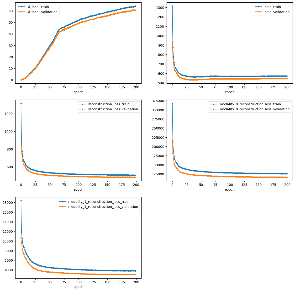
Now, we finally are set and can train the model and visualize the losses.

vae.train()

vae.plot_losses()

Visualizing the latent space

Next, we retrieve the learned latent representation; it is automatically saved in adata.obsm['X_multigrate'].

vae.get_model_output()
adata

AnnData object with n_obs × n_vars = 16433 × 2134
    obs: 'GEX_n_genes_by_counts', 'GEX_pct_counts_mt', 'GEX_size_factors', 'GEX_phase', 'ADT_n_antibodies_by_counts', 'ADT_total_counts', 'ADT_iso_count', 'cell_type', 'batch', 'ADT_pseudotime_order', 'GEX_pseudotime_order', 'Samplename', 'Site', 'DonorNumber', 'Modality', 'VendorLot', 'DonorID', 'DonorAge', 'DonorBMI', 'DonorBloodType', 'DonorRace', 'Ethnicity', 'DonorGender', 'QCMeds', 'DonorSmoker', 'is_train', 'group', 'size_factors', '_scvi_batch'
    var: 'modality'
    uns: 'modality_lengths', '_scvi_uuid', '_scvi_manager_uuid'
    obsm: '_scvi_extra_categorical_covs', 'X_multigrate'
    layers: 'counts'

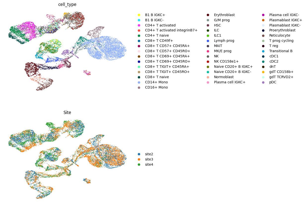
Finally, we visualize the latent space.

sc.pp.neighbors(adata, use_rep="X_multigrate")
sc.tl.umap(adata)

sc.pl.umap(adata, color=["cell_type", "Site"], frameon=False, ncols=1)

Preparing the query

Multigrate is equipped with scArches approach [LNL+22] to map new query data onto existing references.

First, we need to update the model architecture to add weights for the new query batches.

new_vae = mtg.model.MultiVAE.load_query_data(query, reference_model=vae)

Next, we fine-tune the newly added weights to optimize the reconstruction of the query data. We set weight_decay to zero to make sure that the rest of the weights in the model will not be changed.

new_vae.train(weight_decay=0)

Now, we obtain the latent representation of the query and visualize both the reference and the query together.

new_vae.get_model_output(query)
query

AnnData object with n_obs × n_vars = 3567 × 2134
    obs: 'GEX_n_genes_by_counts', 'GEX_pct_counts_mt', 'GEX_size_factors', 'GEX_phase', 'ADT_n_antibodies_by_counts', 'ADT_total_counts', 'ADT_iso_count', 'cell_type', 'batch', 'ADT_pseudotime_order', 'GEX_pseudotime_order', 'Samplename', 'Site', 'DonorNumber', 'Modality', 'VendorLot', 'DonorID', 'DonorAge', 'DonorBMI', 'DonorBloodType', 'DonorRace', 'Ethnicity', 'DonorGender', 'QCMeds', 'DonorSmoker', 'is_train', 'group', 'size_factors', '_scvi_batch'
    var: 'modality'
    uns: 'modality_lengths', '_scvi_uuid', '_scvi_manager_uuid'
    obsm: '_scvi_extra_categorical_covs', 'X_multigrate'
    layers: 'counts'

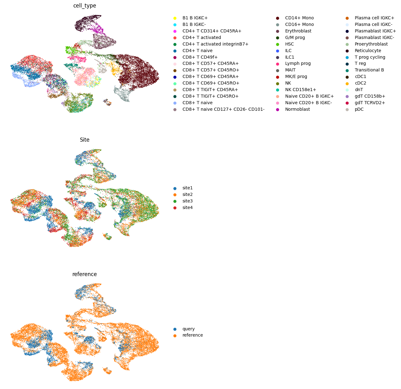
adata.obs["reference"] = "reference"
query.obs["reference"] = "query"
adata_both = ad.concat([adata, query])
adata_both

AnnData object with n_obs × n_vars = 20000 × 2134
    obs: 'GEX_n_genes_by_counts', 'GEX_pct_counts_mt', 'GEX_size_factors', 'GEX_phase', 'ADT_n_antibodies_by_counts', 'ADT_total_counts', 'ADT_iso_count', 'cell_type', 'batch', 'ADT_pseudotime_order', 'GEX_pseudotime_order', 'Samplename', 'Site', 'DonorNumber', 'Modality', 'VendorLot', 'DonorID', 'DonorAge', 'DonorBMI', 'DonorBloodType', 'DonorRace', 'Ethnicity', 'DonorGender', 'QCMeds', 'DonorSmoker', 'is_train', 'group', 'size_factors', '_scvi_batch', 'reference'
    obsm: '_scvi_extra_categorical_covs', 'X_multigrate'
    layers: 'counts'

sc.pp.neighbors(adata_both, use_rep="X_multigrate")
sc.tl.umap(adata_both)

sc.pl.umap(adata_both, color=["cell_type", "Site", "reference"], ncols=1, frameon=False)